Intro
I will (hopefully) get to results of two papers:
- Risk-Budgeted Mean-Variance Portfolios, with Rodrigo Targino and Bernardo da Costa (FGV EMAp)
- What Portfolios Can Risk Budgeting Generate?, with André Santos (CUNEF, Madrid)
Intro
- Portfolio allocation is a central question in Finance
- Two major issues from the practitioner perspective:
- How to model the stochastic process driving returns?
- Given a stochastic process for returns, how to allocate money?
This agenda is mainly about the latter.
The Two Poles
The cornerstone: Mean-Variance (MV)… but nothing comes for free
Mean-Variance (MV)
- ● Best trade-off between risk (variance) and expected returns
- ● Leads to concentrated portfolios
- ● Not very robust to moment estimation error
Risk Budgeting (RB)
- ● Assets control a maximum fraction of the total portfolio risk
- ● Explicit guard against portfolio concentration
- ● No control over expected returns
In the first paper: Risk-Budgeted Mean-Variance (RBMV) portfolio
- RBMV nests both the RB and MV frameworks
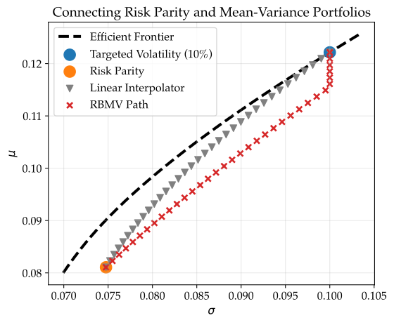
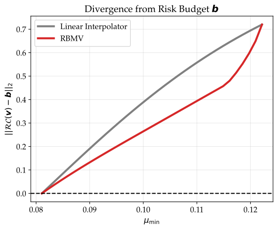
- Makes explicit the tension between expected returns and risk concentration
- Measures how much extra risk concentration you need to accept to get higher returns
Is Risk Budgeting Really Used?
- Risk budgeting was first popularized as Risk Parity (equal risk contributions)
- The term was coined by Qian (2005) at PanAgora
- First commercial product (that I know of): All Weather by Bridgewater in 1996
- Many firms offer risk-budgeting-based products nowadays:
- Some institutional investors directly use it too!
Literature
Mean-Variance
Estimation / Concentration
- Jorion (1986); Black and Litterman (1991)
- Ledoit and Wolf (2003); DeMiguel et al. (2009)
- Jagannathan and Ma (2003)
Risk Budgeting
Flight Plan
- MV and RB: a quick overview
- Our methodology for RBMV
- Empirical application (that I will skip): U.S. equity market using CRSP data
- A glimpse of the results on the second paper: a more theoretical piece!
General takeaway:
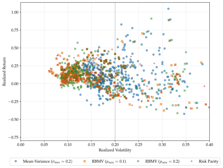
- The RBMV methodology delivers portfolios that are less concentrated than MV …
- But with higher expected returns than RB!
- No way around it: moment estimation is still key
- Second paper: deeper theoretical connection between optimal portfolio choice and RB
MV and RB
Setup
- We trade \(d\) assets indexed by \(i = 1, \ldots, d\)
- Returns \(r_i\) have an expected value \(\mu_{d\times 1}\) and covariance matrix \(\Sigma_{d\times d}\)
- An allocation \(\vv = (v_1, \ldots, v_d)^\intercal\) is a vector of dollars invested in each asset
- You have \(v_0 > 0\) dollars to invest
- The dollar return for an allocation \(\vv\) is given by:
\[ R(\vv) \equiv \sum_{i = 1}^d v_i\cdot r_i = v_0\left[\sum_{i = 1}^d w_i \cdot r_i \right], \qquad w_i \equiv \frac{v_i}{v_0} \]
The MV way
- You want to minimize the variance of returns \(\sigma(R(\vv))\)
- But you request a minimum expected return \(\mu_{\min}^{MV}\)
- The (long-only) MV allocation \(\vv^{MV}\) solves:
\[ \begin{array}[t]{rl} \min\limits_{\vv \geq 0} & \sigma(R(\vv)) \\[0.5ex] \text{s.t.} & \sum_{i=1}^d v_i = v_0 \\[0.5ex] & \mu(R(\vv)) \ge \mu_{\min}^{MV} \cdot v_0 \end{array} \]
- The MV portfolio is given by \(\w^{MV} \equiv \frac{1}{v_0} \cdot \vv^{MV}\)
- This is equivalent to maximizing the return given an upper bound on volatility
Risk Contributions
- If we increase \(v_i\) by $1, how much does the portfolio risk \(\sigma(R(\vv))\) change?
Definition
The risk contribution of asset \(i\) to the total portfolio risk \(\sigma\left(R(\vv)\right)\), is given by: \[\RC_i(\vv) \equiv v_i \cdot \frac{\partial \sigma(R(\vv))}{\partial v_i}\]
- \(\RC_i(\vv)\) is well-defined for every \(\vv \in \R^d_{+}\)
- \(\RC_i(\vv)\) can be high for two reasons: high exposure or high asset volatility
- Since \(\sigma(\cdot)\) is homogeneous of degree 1, Euler’s theorem implies:
\[\sigma(R(\vv)) = \sum_{i=1}^{d}\RC_i(\vv).\]
Risk Budgeting
- RB is designed to limit the risk contributions \(\RC_i(\vv)\)
- We require a (positive) risk budget \(\bb = (b_1, \ldots, b_d)^\intercal\) for total risk and want to invest \(v_0\)
Definition (The Risk Budgeting Portfolio)
The risk budgeting (RB) portfolio is an allocation \(\vv \geq 0\) that satisfies \(v_0 = \sum\limits_{i=1}^{d}v_i\) and \[\frac{\RC_i(\vv)}{\sigma(R(\vv))} = b_i \,, \qquad \text{for all} \quad i=1, \ldots, d\;, \tag{$\star$}\]
- No clue from the definition how to compute \(\vv\)!
- The system in \((\star)\) is a non-linear system of \(d\) equations
How to find this portfolio?
Proposition
Given a positive risk budget \(\bb\), any optimal solution \(\vvstar\) to \[\min_{\vv \in \mathbb{R}^d_+} \sigma(R(\vv))\, , \qquad \text{subject to} \quad \sum_{i = 1}^d b_i \cdot \log(v_i) \ge 0\] is proportional to the exposure \(\vv\) of the RB portfolio for risk budget \(\bb\).
- This problem is strictly convex and easy to solve
- The FOC’s coincide with the RB conditions in \((\star)\)
- We can rescale the solution: \(\displaystyle \vv^{RB} \equiv \frac{v_0}{\sum\limits_{i}^d v_i^*} \vv^*\)
Learning From Simulations
Calibrated Example
- Let \(d = 5\), and \(\bb = (0.2, 0.2, 0.2, 0.2, 0.2)\) – which denotes risk parity
- With population moments, we compute several portfolios:
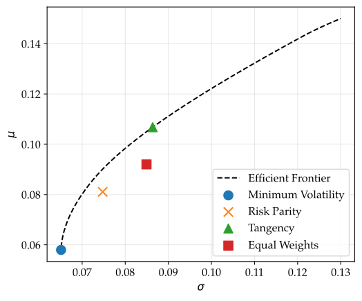
- If all you care is Sharpe Ratio, stick to MV
- Risk parity \(\neq\) Equal weights
- You almost always have to visit the interior to get risk budgeting
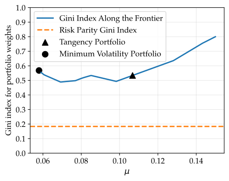
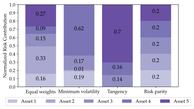
Calibrated Example: Concentration Through the Gini Index
- Given a vector \(\boldsymbol{x} = (x_1, ..., x_n)\), we have \(\text{Gini}(\boldsymbol{x}) \equiv \frac{\sum_{i=1}^{n} \sum_{j=1}^{n} |x_i - x_j|}{2 n \sum_{i=1}^{n} x_i}\).
- \(0 \leq \text{Gini}(\boldsymbol{x}) \leq 1\), and \(\text{Gini}(\boldsymbol{x}) = 0\) if and only if \(\boldsymbol{x}\) is uniform
- Brazilian (wealth) Gini: 0.52; South African Gini: 0.63; Swedish Gini: 0.29
(a) Portfolio weight Gini indices
(b) Risk Contributions
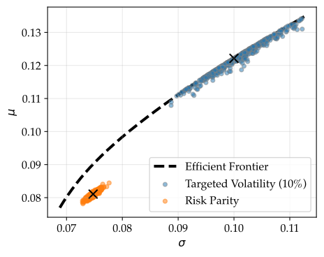
Calibrated Example: Adding Estimation Error
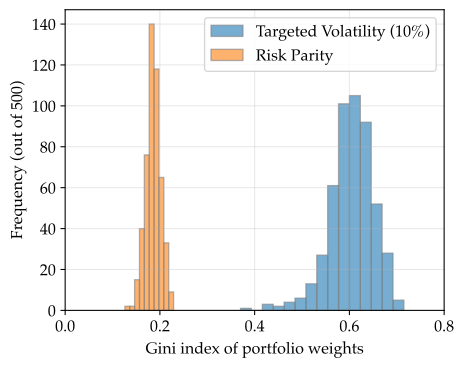
- Simulate 1 year of daily returns, estimate moments, and compute portfolios
- Plot expected returns and vols using the population moments
(a) Simulated portfolios in the \((\sigma, \mu)\)-plane
(b) Distribution of realized Gini indices for \(\w_i\)
Methodology
Our Methodology
Definition (The Risk-Budgeted Mean-Variance Portfolio)
Given a risk budget \(\bb\), an endowment \(v_0\), a minimum required expected return \(\mu_{\text{min}}\), and a maximum volatility bound \(\sigma_{\text{max}}\), the Risk Budgeted Mean-Variance Portfolio (RBMV) is given by \(\vv = \frac{v_0}{\sum_{i=1}^{d}v_i^*}\cdot \vv^*\), where \(\vv^*\) is the solution of: \[ \begin{array}[t]{rll} \min\limits_{\vv \in \mathbb{R}^d_{+}} & \sigma(R(\vv)) \\[0.5ex] \text{s.t.} & \sum\limits_{i=1}^d b_i \log(v_i) \ge 0 & \quad [\lambda_v] \\[0.5ex] & \mu(R(\vv)) \ge \mu_{\min} \sum_{i=1}^d v_i & \quad [\lambda_\mu] \\[0.5ex] & \sigma(R(\vv)) \le \sigma_{\max} \sum_{i=1}^d v_i\, , & \quad [\lambda_\sigma] \end{array} \] The corresponding portfolio weights are given by \(\w = \frac{1}{v_0}\vv\).
Our Methodology: First-Order Conditions
Put every constraint in \(\ge 0\) form and attach its multiplier:
\[ \begin{aligned} \mathcal{L}(\vv; \lambda_v, \lambda_\mu, \lambda_\sigma) \;=\;& \sigma(R(\vv)) \;-\; \lambda_v \Big[\textstyle\sum_{i} b_i \log v_i\Big] \\[0.35em] &-\; \lambda_\mu \Big[\mu^\intercal \vv - \mu_{\min}\boldsymbol{1}^\intercal \vv\Big] \;-\; \lambda_\sigma \Big[\sigma_{\max}\boldsymbol{1}^\intercal \vv - \sigma(R(\vv))\Big] \end{aligned} \]
\[ \frac{\partial \mathcal{L}}{\partial v_i} = \frac{\partial \sigma(R(\vv))}{\partial v_i} - \lambda_v \frac{b_i}{v_i} - \lambda_\mu\left(\mu_i - \mu_{\min}\right) - \lambda_\sigma\left(\sigma_{\max} - \frac{\partial \sigma(R(\vv))}{\partial v_i}\right) = 0 \]
- If neither the return floor nor the vol cap binds, slackness gives \(\lambda_\mu = \lambda_\sigma = 0\):
\[ \underbrace{v_i \cdot \frac{\partial \sigma(R(\vv))}{\partial v_i}}_{\equiv\RC_i(\vv) } \;=\; \lambda_v\, b_i \]
- But \(\sum_i b_i = 1\), so \(\lambda_v = \sigma(R(\vv))\):
\[ \RC_i(\vv) = b_i \cdot \sigma(R(\vv)), \qquad i = 1, \ldots, d \implies \quad \text{We nest the RB solution!} \]
Our Methodology: The Lagrangian View
\[ \frac{\partial \mathcal{L}(\vv; \lambda_v, \lambda_\mu, \lambda_\sigma)}{\partial v_i} = \frac{\partial \sigma(R(\vv))}{\partial v_i} - \lambda_v \frac{b_i}{v_i} - \lambda_\mu \left(\mu_i - \underbrace{\mu_{\text{min}}}_{\color{red}{\text{moves around}}}\right) - \lambda_\sigma \left(\underbrace{\sigma_{\text{max}}}_{=0.1} - \frac{\partial \sigma(R(\vv))}{\partial v_i}\right) \]
Empirical Application
Empirical Application
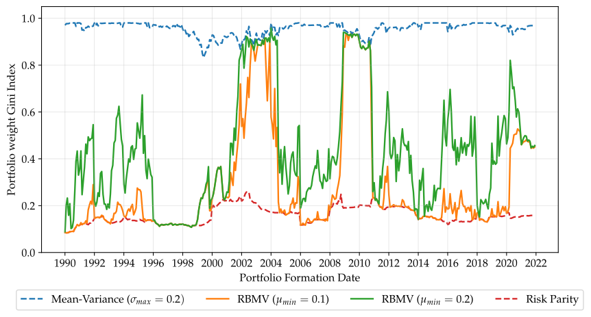
- Every month, we build a long-only portfolio with the 50 largest stocks in the U.S.
- Sample: 1990-2023
- Estimate population moments \(\hat{\mu}\) and \(\hat{\Sigma}\) with 2 years of historical data (CRSP)
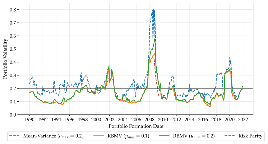
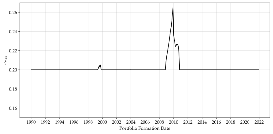
- Solve for the minimum vol portfolio and set \(\sigma_{max} = \min\{\sigma_{MinVol} + 0.02, 0.2\}\)
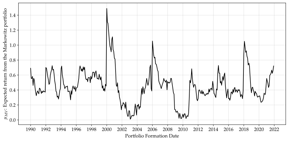
- Find the MV portfolio with the highest returns, given \(\sigma_{max}\)
- Set two possible values for \(\mu_{min}\):
\[ \begin{aligned} \mu_{min,\ \text{conservative}} &\equiv \min\{\mu_{MV} - 0.05, 0.1\}\\ \mu_{min,\ \text{greedy}} &\equiv \min\{\mu_{MV} - 0.05, 0.2\} \end{aligned} \]
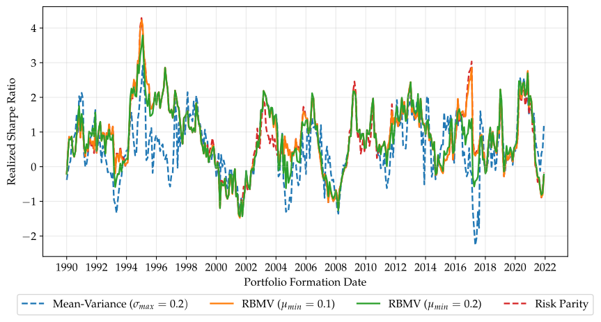
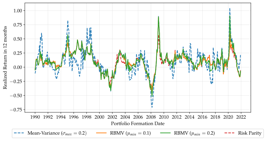
- Hold 4 portfolios for 1 year: Risk Parity, MV(\(\sigma_{max}\)), RBMV(\(\mu_{min, \text{conservative}}; \sigma_{max}\)), and RBMV(\(\mu_{min, \text{greedy}}; \sigma_{max}\))
Realized Gini Index
Annualized Standard Deviation of Daily Returns
Portfolios in the \((\sigma, \mu)\)-Plane
Average results
Full Sample (1990-2022)
| Portfolio | Return (%) | Volatility (%) | Sharpe Ratio | Gini Index (\(\w_i\)) |
|---|---|---|---|---|
| Risk Parity | 9.68 | 15.69 | 0.84 | 0.16 |
| RBMV (\(\mu_{min}=0.1\), \(\sigma_{max}=0.2\)) | 10.29 | 15.98 | 0.86 | 0.29 |
| RBMV (\(\mu_{min}=0.2\), \(\sigma_{max}=0.2\)) | 10.50 | 16.70 | 0.81 | 0.43 |
| Mean-Variance (\(\sigma_{max}=0.2\)) | 10.20 | 22.28 | 0.58 | 0.96 |
- We were able to tilt the Risk Parity portfolio towards higher returns
- Just a bit more of concentration led to higher returns and slightly higher SR
- The MV portfolio was invested in just a few assets!
What Can Risk Budgeting Generate?
A New Question
- Work with weights of fully invested, long-only portfolios:
\[ \Delta_d^\circ = \{\w \in \R^d_{++} : \boldsymbol{1}^\intercal \w = 1\}, \qquad \mathcal{B}^\circ = \{\bb \in \R^d_{++} : \boldsymbol{1}^\intercal \bb = 1\} \]
- \(\w\) is an RB portfolio for budget \(\bb \in \mathcal{B}^\circ\) when:
\[ \RC_i(\w) = b_i \cdot \sigma(\w) \quad \Longleftrightarrow \quad \frac{w_i (\Sigma \w)_i}{\w^\intercal \Sigma \w} = b_i, \qquad i = 1, \ldots, d \]
- Forward problem: given \(\bb\), compute \(\w = G(\bb)\); well defined under \(\Sigma \succ 0\)
- Inverse question: which portfolios come out as \(\bb\) varies over \(\mathcal{B}^\circ\)?
\[ \mathcal{I} \equiv G(\mathcal{B}^\circ) \subseteq \Delta_d^\circ \qquad \textit{Is this inclusion strict? When?} \]
The Image of Positive Risk Budgeting
Theorem (Image)
A portfolio \(\w \in \Delta_d^\circ\) belongs to \(\mathcal{I}\) if and only if \(\Sigma \w > 0\) componentwise. Hence \[\mathcal{I} = \Delta_d^\circ \cap \{\w \in \R^d : \Sigma \w > 0\}.\]
Theorem (Completeness)
The positive risk-budgeting map is complete, i.e., \(\mathcal{I} = \Delta_d^\circ\), if and only if \(\Sigma\) is entrywise nonnegative.
- A single \(\sigma_{ij} < 0\) implies: portfolios close enough to asset \(j\) make asset \(i\) a hedge
- Example: one-factor model with same-sign loadings (\(\Sigma = \sigma_f^2 \beta \beta^\intercal + D\))
- The signs of \(\beta\) determine completeness (or lack thereof)
Risk Budgets Are Weight-Scaled Betas
Recall: the beta of asset \(i\) w.r.t. the portfolio is \(\beta_{i,p}(\w) \equiv \frac{(\Sigma \w)_i}{\w^\intercal \Sigma \w}\), with \(\sum\limits_{i=1}^{d}w_i\cdot\beta_{i,p} = 1\)
Proposition (Risk budgets are weight-scaled betas)
For every \(\w \in \mathcal{I}\): \[b_i(\w) = w_i \cdot \beta_{i,p}, \qquad i = 1, \ldots, d.\]
- A risk budget is not a capital weight: it is a slice of the portfolio’s own beta
- Equal budgets \(\Rightarrow\) high-beta assets get smaller weights
Diversification is not insurance:
- A held asset with \(\beta_{i,p} < 0\) is insurance: its risk contribution is negative
- Positive budgets ask every contribution to be positive!
- Examples: hedge sleeves (small amounts of Treasuries, gold, tail hedges)
Recall: How to Microfound MV?
- CARA investor: \(U(W) = -\exp(-\gamma W)\), \(\gamma > 0\); normalize \(v_0 = 1\), so \(W = 1 + \w^\intercal \boldsymbol{r}\)
- Gaussian returns: \(\w^\intercal \boldsymbol{r} \sim \mathcal{N}\left(\mu^\intercal \w,\; \w^\intercal \Sigma \w\right)\)
- The MGF of a Gaussian gives:
\[\E[U(W)] = -e^{-\gamma}\cdot\exp\left(-\gamma\, \mu^\intercal \w + \tfrac{1}{2}\gamma^2\, \w^\intercal \Sigma \w\right)\]
- Maximizing \(\E[U(W)]\) is equivalent to:
\[\max_{\w \in \Delta_d} \quad \mu^\intercal \w - \gamma\, \w^\intercal \Sigma \w\]
- Gaussianity collapses the distribution to \((\mu, \Sigma)\); CARA makes initial wealth irrelevant
- \(\gamma\) is not just a dial: it is the risk aversion of a specific agent
- Restrictions on \(\gamma\) = restrictions on whose preferences a portfolio can reflect
Which MV Investors Can Risk Budgeting Mimic?
- For a given \(\gamma > 0\), define the active set: \(S_\gamma \equiv \{i : w_i(\gamma) > 0\}\)
- FOCs deliver a scalar \(\lambda_\gamma > 0\) such that \(\mu_i - 2\gamma (\Sigma \w(\gamma))_i = \lambda_\gamma\), for all \(i \in S_\gamma\)
- \(\w(\gamma)\) is RB-rationalizable if some positive budget \(\bb \in \mathcal{B}^\circ\) generates it, i.e., \(\w(\gamma) \in \mathcal{I}\)
Theorem (MV portfolios in the RB image)
The portfolio \(\w(\gamma)\) is RB-rationalizable if and only if every held asset earns more than the zero-beta intercept: \[\min_{i \in S_\gamma} \mu_i > \lambda_\gamma.\]
- MV allows assets as return producers or as insurance; RB only admits the first role
Risk Budgeting as High-Risk-Aversion Mean-Variance
Theorem (Risk-aversion threshold)
Fix an active set \(S\). While \(S_\gamma = S\), there is a threshold \(\overline{\gamma}^{RB}_S\), depending only on \((\mu, \Sigma, S)\), such that \[\w(\gamma) \text{ is RB-rationalizable} \quad \Longleftrightarrow \quad \gamma > \overline{\gamma}^{RB}_S.\]
- Below \(\overline{\gamma}_S^{RB}\), the investor optimally buys insurance
- As \(\gamma \to \infty\), you buy so much insurance that it is not insurance anymore!
- Example: gold can be a hedge only if you do not own a gold mine!
Takeaway
Choosing risk budgeting is like behaving as a mean-variance investor with sufficiently high risk aversion!
Discussion and Extensions
Risk Measures Beyond Volatility
- Let \(\rho(\vv) \equiv \rho(R(\vv))\) be a portfolio risk measure
- The key property for risk budgeting is positive homogeneity
\[\rho(\gamma \vv) = \gamma \rho(\vv), \qquad \gamma > 0.\]
- Prime example: Expected Shortfall on losses \(L(\vv) = -R(\vv)\)
\[\ES_\alpha(L(\vv)) = \E\left[L(\vv)\mid L(\vv) \geq \VaR_\alpha(L(\vv))\right].\]
- For any \(\rho\) with a reasonable concept of gradient, define risk contributions \(\RC_i^\rho(\vv) \equiv v_i \frac{\partial \rho(\vv)}{\partial v_i}\)
- Euler’s theorem gives the same risk-decomposition logic:
\[\rho(\vv) = \sum_{i=1}^{d} \RC_i^\rho(\vv).\]
Short Sales: What Breaks?
- Long-only RB/RBMV uses positive dollar exposures:
\[ \RC_i^\rho(\vv) \equiv v_i \frac{\partial \rho(\vv)}{\partial v_i}, \qquad b_i \rho(\vv) = \RC_i^\rho(\vv) \]
\[\sum_i b_i \log(v_i) \geq 0.\]
- If \(v_i < 0\), then \(\log(v_i)\) is undefined
- \(\RC_i^\rho(\vv)\) can be negative, so it is no longer a positive share of total risk
- \(\sum_i v_i = v_0\) becomes net exposure, not the size of the long/short book.
We cannot just remove the constraint \(\vv \geq 0\).
Short Sales: Fix Signs
- Let the investor fix the signs before optimization:
\[s_i \in \{-1,+1\}, \qquad x_i > 0, \qquad v_i = s_i x_i.\]
- \(s_i=-1\) means asset \(i\) is chosen in advance to be short
- Budget risk over position magnitudes \(\boldsymbol{x}\):
\[ \begin{aligned} R_s(\boldsymbol{x}) &\equiv R(\boldsymbol{s}\odot\boldsymbol{x}) = \sum_{i=1}^d s_i x_i r_i, \\ \widetilde{\RC}_i(\boldsymbol{x}) &\equiv x_i \frac{\partial \rho(R_s(\boldsymbol{x}))}{\partial x_i}. \end{aligned} \]
Short Sales: Budget Magnitudes
- Once signs are fixed, homogeneity works in the magnitudes:
\[\rho(R_s(\boldsymbol{x})) = \sum_{i=1}^d \widetilde{\RC}_i(\boldsymbol{x}).\]
- The log formulation is also well-defined because \(x_i>0\):
\[ \min_{\boldsymbol{x}\in\mathbb{R}_{++}^d}\quad \rho(R_s(\boldsymbol{x})) \quad \text{s.t.} \quad \sum_{i=1}^d b_i \log(x_i) \geq 0. \]
Easy once signs are fixed; hard if the model must choose what to short.
Conclusion
Wrap-Up:
- MV is the cornerstone of portfolio allocation, but leads to high concentration
- RB tackles concentration at the expense of expected returns
- RBMV nests both, and allows you to control this trade-off in a transparent way
- A Julia package for fast implementation: RiskBudgetingMeanVariance.jl
- Diversification is not hedging … we are at the infancy of understanding RB
Going forward:
- Some extensions: short-selling, transaction costs, …
- What kind of other markets can benefit from this methodology? What examples are interesting?
Appendix
Appendix and References
Calibration Details
We assume \(d=5\) and use the following population moments for the mean returns \(\mu\), the individual standard deviations \(s\) and correlation matrix \(C\):
\[ \mu = \begin{bmatrix} 0.5 \\ 0.12 \\ 0.09 \\ 0.05 \\ 0.15 \end{bmatrix}, \quad s = \begin{bmatrix} 0.10 \\ 0.20 \\ 0.15 \\ 0.08 \\ 0.13 \end{bmatrix}, \quad C = \begin{bmatrix} 1 & 0.20 & 0.40 & 0.25 & 0.50\\ 0.20 & 1 & -0.20 & 0.40 & 0.6\\ 0.40 & -0.20 & 1 & -0.10 & 0.30\\ 0.25 & 0.40 & -0.10 & 1 & 0.30\\ 0.50 & 0.60 & 0.30 & 0.30 & 1 \end{bmatrix} \]
We further define \(\Sigma \equiv s^\intercal C s\).
Realized Sharpe Ratio
Realized Returns
Actual Maximal Volatility
Expected Return From The MV Approach
Alternative Samples
Panel B: Before the Great Financial Crisis (1990-2006)
| Portfolio | Return (%) | Volatility (%) | Sharpe Ratio | Gini Index (\(\w_i\)) |
|---|---|---|---|---|
| Risk Parity | 10.79 | 14.42 | 0.89 | 0.15 |
| RBMV (\(\mu_{min}=0.1\), \(\sigma_{max}=0.2\)) | 10.90 | 14.45 | 0.91 | 0.26 |
| RBMV (\(\mu_{min}=0.2\), \(\sigma_{max}=0.2\)) | 10.74 | 14.99 | 0.85 | 0.39 |
| Mean-Variance (\(\sigma_{max}=0.2\)) | 9.92 | 20.84 | 0.50 | 0.95 |
Panel C: After 2020 (2021-2022)
| Portfolio | Return (%) | Volatility (%) | Sharpe Ratio | Gini Index (\(\w_i\)) |
|---|---|---|---|---|
| Risk Parity | 0.07 | 15.65 | 0.21 | 0.16 |
| RBMV (\(\mu_{min}=0.1\), \(\sigma_{max}=0.2\)) | 0.93 | 16.00 | 0.27 | 0.46 |
| RBMV (\(\mu_{min}=0.2\), \(\sigma_{max}=0.2\)) | 1.52 | 16.01 | 0.30 | 0.47 |
| Mean-Variance (\(\sigma_{max}=0.2\)) | 12.62 | 16.31 | 0.84 | 0.96 |